Visualization Methodology
This text describe the methodology that DOSPORTAL uses to visualize data.
Evolution Charts
Vizualize dosimetric data in time.
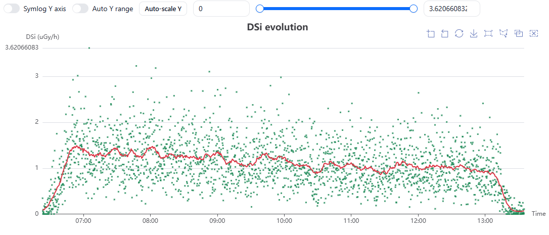
Absorbed dose rate in silicon over the course of a measurement.
Absorbed dose rate in silicon
Absorbed dose in silicon $D_{\mathrm{Si}}$ quantifies the energy absorbed by ionizing radiation per unit mass of silicon. The absorbed dose rate in silicon $\dot{D}_{\mathrm{Si}}$ expresses this quantity per unit time.
\[\dot{D}_{Si} = \frac{E_j \, q}{m} \cdot \frac{10^{6} \cdot 3600}{\Delta t} \quad [\mathrm{\mu Gy/h}]\]The absorbed dose rate in silicon is calculated in three steps for each measurement:
1. Channel-energy calibration
\[E_j = \mathrm{coef_0} + \mathrm{coef_1} \cdot j \quad [\mathrm{MeV}],\]where $j$ is the channel number and $\mathrm{coef_0}$ and $\mathrm{coef_1}$ are detector-specific energy calibration coeficients.
2. Deposited energy
\(E = \sum_{j=j_0} C_{j}(t)\,E_j \quad [\mathrm{MeV}],\) where $C_{j}$ is the number of counts in channel $i$ during the measurement. $j_0$ is the first channel included in the calculation. E.g. for some AIRDOS detectors, the first four channels are excluded as they are dominated by the noise signal.
3. Absorbed dose rate in silicon. The energy is converted to joules, divided by the detector-specific mass $m$ of the sensitive silicon volume and expressed per hour:
\[\dot{D}_{Si} = \frac{E \cdot q}{m} \cdot \frac{10^{6} \cdot 3600}{\Delta t} \quad [\mathrm{\mu Gy/h}],\]where
$\Delta t$ is the integration time of the measurement. For AIRDOS detectors, the $\Delta t$ is typically 10.4 s,
$q = 1.602176634 \times 10^{-13}$ is a constant converting MeV to J,
$10^6$ is constant converting the unit Gy to µGy, and
$3600$ is constant converting seconds to hours.
Red line
The red line is a centered moving average over 50 exposures, for the AIRDOS detectors this corresponds to approximately 520 s 8 minutes and 40 seconds.
Flux evolution
The particle flux for each exposure is calculated from the number of registered events, normalized by the sensitive area of the silicon detector $S$ and the exposure duration $\Delta t$: \(\dot{\Phi}_i = \frac{n_i}{S \cdot \Delta t} \qquad [\mathrm{cm^{-2}\,s^{-1}}],\)
where $n_i$ is the total number of events registered during exposure $i$:
\[n_i = \sum_{j=j_{\min}} C_{i,j},\]$C_{i,j}$ is the number of events registered in energy channel $j$ during exposure $i$, $j_{\min}$ is the first channel included in the calculation.
For some AIRDOS detectors, the first four channels are excluded because they are dominated by noise, corresponding to $j_{\min}=4$. The exposure duration $\Delta t$ is detector-specific; for AIRDOS detectors it is typically 10.4 s.
Red line
The red line represents a centered moving average over 50 exposures. For an exposure duration of 10.4 s, this corresponds to approximately 520 s, or 8 min 40 s.
Count Evolution
Registered event count per exposure.
For each exposure $i$, the displayed value is
\[y_i = {n_i},\]where the total number of registered events $n_i$ is calculated as
\[n_i = \sum_{j=j_{\min}} C_{i,j},\]where, and $j_{\min}$ is the first channel included in the calculation. For some AIRDOS detectors, $j_{\min}=4$, meaning that the first four channels are excluded because they are dominated by noise. Unlike the particle flux, the event count is not normalized by the detector area or exposure duration.
Red line
The red line represents a centered moving average over 50 exposures. For an exposure duration of 10.4 s, this corresponds to approximately 520 s, or 8 min 40 s.
Spectrum Charts
Spectrum charts show the distribution of registered events across detector channels or corresponding deposited-energy bins.
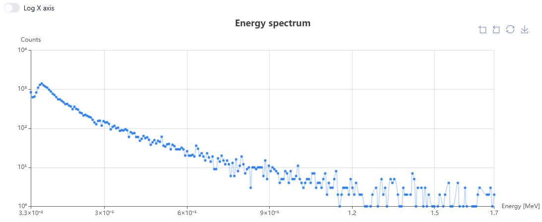
Energy Spectrum.
Energy Spectrum
The energy spectrum shows the number of registered events $\sum_i C_{i,j}$ in channel $j$ as a function of deposited energy $E_j$. The sum is performed over all exposures included in the selected time interval. Only channels with $j \geq j_{\min}$ are included in the spectrum.
Energy spectrum organize data by energy levels.
Two step process described below:
1. Sum over exposures
For each channel, the registered events are summed over all selected exposures $i$:
\[y_j = \sum_i C_{i,j} \qquad [\mathrm{counts}].\]2. Channel-energy calibration
The channel number is converted to the corresponding deposited energy using the selected detector calibration:
\[E_j = \mathrm{coef}_0 + (j)\,\mathrm{coef}_1 \qquad [\mathrm{MeV}],\]where $\mathrm{coef}_0$ and $\mathrm{coef}_1$ are detector-specific calibration coeficients.
Channel Spectrum
The channel spectrum shows the number of registered events $\sum_i C_{i,j}$ as a function of detector channel $j$. The sum is performed over all exposures included in the selected time interval. Only channels with $j \geq j_{\min}$ are included. For some AIRDOS detectors, $j_{\min}=4$ because the first four channels are dominated by noise.
Time window
Selected time intervals can be used for further analysis.
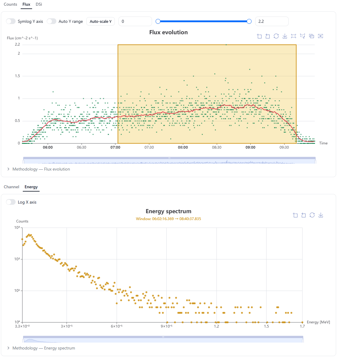
Time window selected by the user.
Blue: spectrum accumulated over the full measurement interval (default view).
Yellow: spectrum accumulated over the selected time window. When a time window is selected, its spectrum is shown in the accent colour and the full-measurement spectrum is hidden.
Dosimetric quantities
The following quantities are reported for the selected window:
- $\overline{\dot{D}_{\mathrm{Si}}}$ — mean absorbed dose rate $[\mathrm{\mu Gy/h}]$
- $\sigma_{\dot{D_{Si}}}$ — sample standard deviation of the absorbed dose rate $[\mathrm{\mu Gy/h}]$
- $D_{\mathrm{Si}}$ — absorbed dose accumulated over the selected window $[\mathrm{\mu Gy}]$
- $T$ — duration of the selected window $[\mathrm{h}]$
- $N$ — number of dose-rate measurements included in the selected time window
1. Mean absorbed dose rate
The absorbed dose rates of all exposures included in the selected window are averaged:
\(\overline{\dot{D}_{\mathrm{Si}}} = \frac{1}{N} \sum_{i \in W} \dot{D}_{\mathrm{Si},i} \qquad [\mathrm{\mu Gy/h}],\) where $W$ is the set of exposures included in the selected time window, $N$ is the number of exposures in the selected time window.
2. Variation of the absorbed dose rate
The sample standard deviation of the absorbed dose rates in silicon $\sigma_{\dot{D_{Si}}}$ within the selected window is calculated as
\(\sigma_{\dot{D_{Si}}} = \sqrt{ \frac{1}{N-1} \sum_{i \in W} \left( \dot{D}_{\mathrm{Si},i} - \overline{\dot{D}_{\mathrm{Si}}} \right)^2 } \qquad [\mathrm{\mu Gy/h}],\) where $\dot{D}_{\mathrm{Si},i}$ is the absorbed dose rate in silicon for exposure $i$, calculated as described in Absorbed dose rate in silicon.
For a window containing a single exposure ($N=1$), the standard deviation is reported as $0$.
3. Window duration and accumulated dose
The selected window boundaries are stored in milliseconds and converted to hours:
\(T = \frac{t_{\mathrm{max}} - t_{\mathrm{min}}} {3.6 \times 10^6} \qquad [\mathrm{h}],\) where $t_{\mathrm{min}}$ and $t_{\mathrm{max}}$ are the boundaries of the selected time window in milliseconds and $3.6 \times 10^6$ converts milliseconds to hours.
If the measurement continuously covers the selected time window, the accumulated absorbed dose is
\[D_{\mathrm{Si}} = \overline{\dot{D}_{\mathrm{Si}}}\,T \qquad [\mathrm{\mu Gy}].\]Note: $T$ represents the duration between the selected time boundaries and not necessarily the sum of the individual exposure durations $\Delta t$.